北京邮电大学鲁鹏《计算机视觉(本科)》笔记
注:
- 评价:
- 课程视频 计算机视觉(本科) 北京邮电大学 鲁鹏
- 课程资料 CV-XUEBA
- 课程大概
image.png
概述
-
David Marr 三层问题方法论 (ICCV马尔奖)
- Computational theory: What is the goal of the computation (task) and what are the constraints that are known or can be brought to bear on the problem?
- Representations and algorithms: How are the input, output, and intermediate information represented, and which algorithms are used to calculate the desired result?
- Hardware implementation: How are the representations and algorithms mapped onto actual hardware, Conversely, how can hardware constraints be used to guide the choice of representation and algorithm?
-
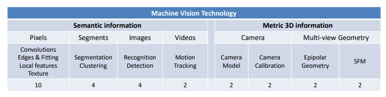
information extracted from an image
- Metric 3D information
- Semantic information
-
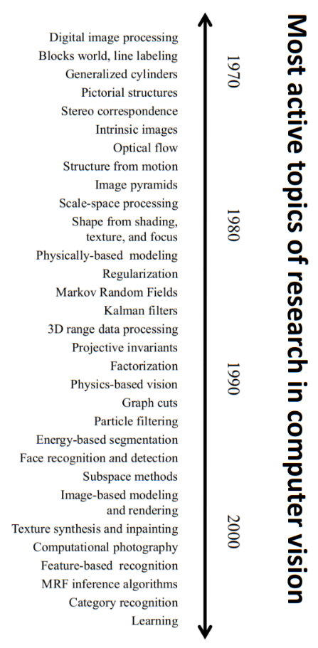
CV发展时间表
语义信息
像素
卷积
- 卷积核(滤波核)
- …省略
- 去噪:高斯平滑(线性)解决高斯噪声,中值滤波(非线性)解决椒盐噪声
- 锐化
边缘提取
-
偏导
-
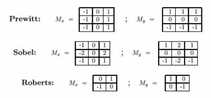
检测边缘的特殊滤波核(sobel先高斯平滑再提取)
-
有噪声,先平滑
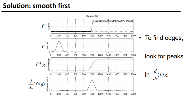
image.png 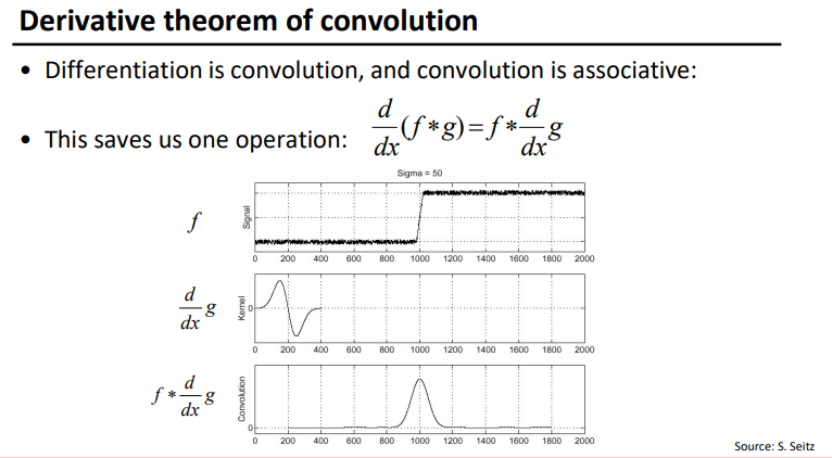
image.png -
Smoothing vs. derivative filters
- Gaussian: remove “high-frequency” components; “low-pass” filter
- the values of a smoothing filter Cannot be negative
- the values sum to 1
- One: constant regions are not affected by the filter
-
Derivative filters
- Derivatives of Gaussian
- the values of a derivative filter Can be negative
- the values sum to 0
- High absolute value at points of high contrast
-
Non-maximum suppression 非最大化抑制
- 宽边变细边
- Check if pixel is local maximum along gradient direction, select single max across width of the edge
-
Hysteresis thresholding 滞后阈值法
- Use a high threshold to start edge curves, and a low threshold to continue them.
-
Canny edge detector算法
- Filter: derivative of Gaussian
- Find magnitude and orientation of gradient
- Non-maximum suppression:
- Linking and thresholding (hysteresis)
拟合
-
需要数学描述轮廓位置
-
Least squares最小二乘
- 缺点:Not rotation-invariant 没有旋转不变性、Fails completely for vertical lines垂直
- 改进:Total least squares, TLS,总体最小二乘法(有点类似svm)(点到直线垂直距离)
- 【略去数学】
- 求解Ax=b的最小二乘法只认为b含有误差,但实际上系数矩阵A也含有误差。总体最小二乘法就是同时考虑A和b二者的误差和扰动
- 改进:Robust fitting(有点类似正则化)距离超过某个值不考虑
-
Random sample consensus(RANSAC)
- 很多外点的时候有用
- 步骤
- Choose a small subset of points uniformly at random
- Fit a model to that subset
- Find all remaining points that are “close”(确定门限) to the model and reject the rest as outliers
- Do this many times and choose the best model
-
Hough transform
-
投票机制
-
换成极坐标,避免垂直时参数失效(theta可以根据导数计算,缩小搜索范围)
-
步骤
- Discretize parameter space into bins
- For each feature point in the image, put a vote in every bin in the parameter space that could have generated this point
- Find bins that have the most votes
-
Dealing with noise
- Choose a good grid / discretization
- Too coarse: large votes obtained when too many different lines correspond to a single bucket
- Too fine: miss lines because some points that are not exactly collinear cast votes for different buckets
- Increment neighboring bins (smoothing in accumulator array)(给周边格子加分)
- Try to get rid of irrelevant features (Take only edge points with significant gradient magnitude)
- Choose a good grid / discretization
-
Hough transform for circles
-
找样本一点,求梯度方向,方向上各个根据x,y,转换到r,u,v坐标系,设定三维坐标系投票
-
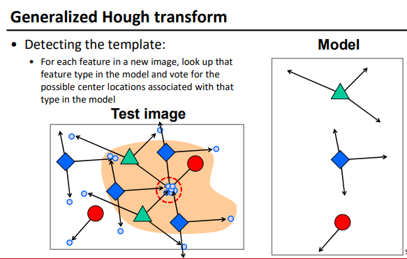
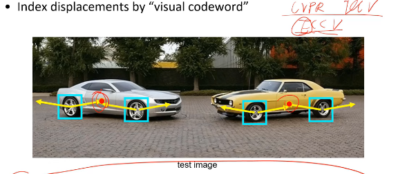
拓展
-
-
优点
- Can deal with non-locality全局 and occlusion遮挡
- Can detect multiple instances of a model多物体
- Some robustness to noise: noise points unlikely to contribute consistently to any single bin
-
缺点
- Complexity of search time increases exponentially with the number of model parameters 高维度很难
- Non-target shapes can produce spurious peaks in parameter space 伪峰值
- It’s hard to pick a good grid size 离散化的标准不确定
-
-
Hough transform vs. RANSAC
- Hough变换的优点是概念简单(只需变换和在Hough空间中找到交叉点)。它也相当容易实现,并且可以很好地处理丢失和阻塞的数据。另一个优点是,只要结构具有参数方程,它就可以找到除直线以外的其他结构。 缺点包括在参数越多,计算上越复杂。它也只能同时查找一种结构(因此不能将线和圆放在一起)。也不能检测到线段的长度和位置。它可以被“明显”的线条欺骗,并且不能同线性的线段作区分。
- RANSAC 每次一条线或者最多的几条线 投票 外点数越多越麻烦 计算参数的迭代次数没有上限
局部特征
角 Corner
-
图像拼接过程
- extract features
- match features
- align images
-
找关键点的注意事项
- Repeatability 可重复性 - The same feature can be found in several images despite geometric and photometric transformations
- Saliency 要有特点 - Each feature is distinctive
- Compactness and efficiency 简洁有效率 - Many fewer features than image pixels
- Locality 局部性 - A feature occupies a relatively small area of the image; robust to clutter and occlusion
-
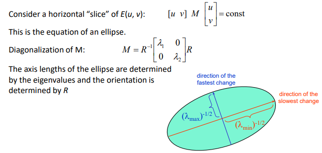
计算挪动坐标后窗口内差异值
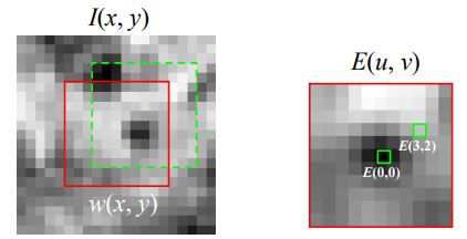
image-20220907133251325 泰勒展开
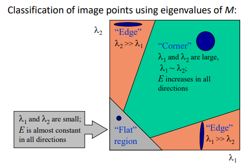
只要两个特征值都比较大就可以认为是角点
-
M<两个特征值反应两个方向上变化的强弱>,R表现旋转角度
-
Harris detector 步骤
- Compute Gaussian derivatives at each pixel
- Compute second moment matrix M in a Gaussian window around each pixel
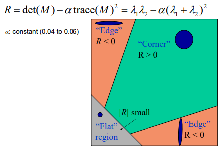
- Compute corner response function R
- Threshold R
- Find local maxima of response function (nonmaximum suppression) 要有非最大化抑制
-
Harris角点特性
-
Invariance不变: image is transformed and corner locations do not change 直接建立关联
-
Affine intensity change (放射强度变换,亮度) Partially invariant to affine intensity change 部分满足
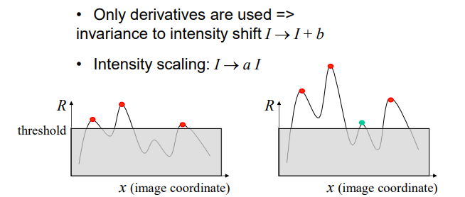
image-20220907162134681
-
-
Covariance协变: if we have two transformed versions of the same image, features should be detected in corresponding locations 有机会建立关联
-
对于平移、旋转、放大:
-
平移:Derivatives and window function are shift-invariant
-
旋转:Second moment ellipse rotates but its shape (i.e. eigenvalues) remains the same
-
放大:All points will be classified as edges. Corner location is not covariant to scaling!
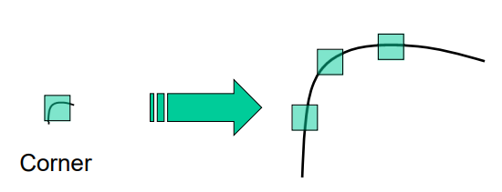
image-20220907162148380
-
-
-
斑点(圆)检测 Blob
-
Goal: independently detect corresponding regions in scaled versions of the same image
-
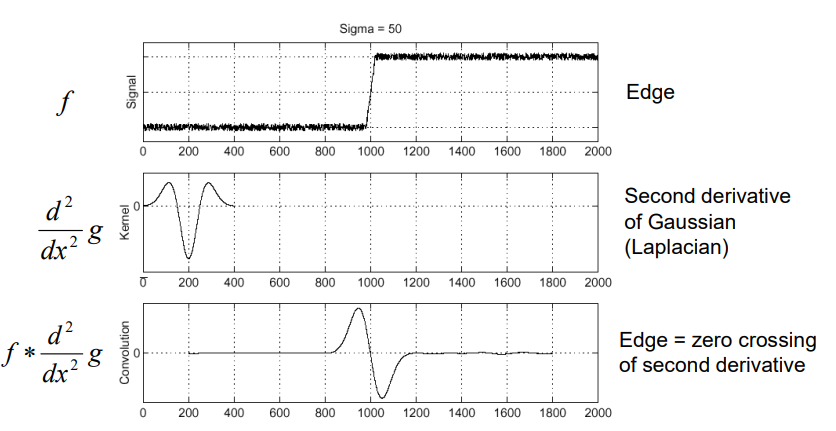
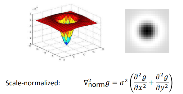
高斯二阶导,拉普拉斯
-
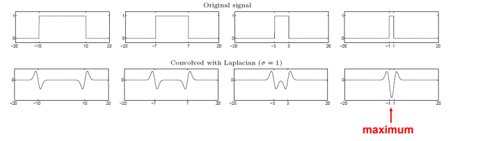
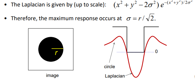
Blob = superposition of two ripples 两个边缘的叠加
-
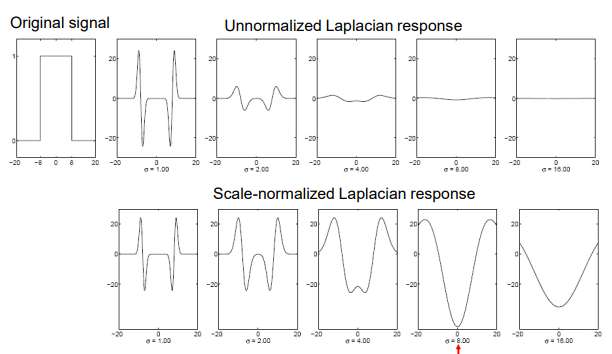
Spatial selection: the magnitude of the Laplacian response will achieve a maximum at the center of the blob, provided the scale of the Laplacian is “matched” to the scale of the blob
-
sigma增大会使得响应衰减需要乘上sigma平方修正
-
二维
-
圆半径和sigma如何匹配(首先尺寸问题)
-
define the characteristic scale of a blob as the scale that produces peak of Laplacian response in the blob center
-
增强方法:DoG算子本质是为了LoG算子的快速实现。其通过两个高斯的差快速逼近了LoG算子
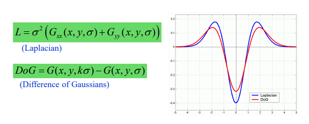
没听懂 p8 52min左右 大概是sigma不变 改k就行
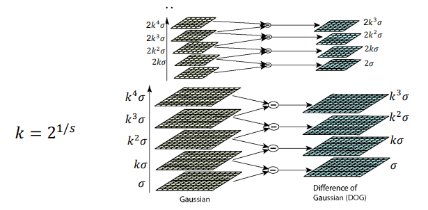
image-20220907201709381 -
Laplacian (blob) response 点is invariant w.r.t. rotation and scaling
-
Blob location and scale is covariant w.r.t. rotation and scaling
-
修正
-
视角问题:类比Harris的方法找出两个方向变化相等的时候,图像上时椭圆,特征向量的图是正圆
-
旋转问题:局部合到整体投票,根据最大旋转角统一两幅图的方向
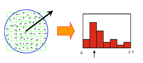
image-20220907205809764 -
光照问题:分成局部,两幅图的每个对应局部的光强直方图进行L2距离比较
-
-
纹理
-
Texture representations attempt to summarize repeating patterns of local structure
-
Filter banks useful to measure redundant variety of structures in local neighborhood
-
使用Filter banks (Feature spaces can be multi-dimensional) 非常类似卷积最后提取的特征
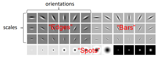
image-20220908110450033
分割
- 对于本节:Bottom-up process & Unsupervised
基于kmeans
- Pros
- Very simple
- Converges to a local minimum of the error function 收敛到误差函数的局部最小值
- Cons
- Memory-intensive 内存密集型
- Need to pick K
- Sensitive to initialization
- Sensitive to outliers
- Only finds “spherical” clusters
基于Mean shift
-
eg (r,g,b,x,y)
-
Pros
- Does not assume spherical clusters
- Just a single parameter (window size)
- Finds variable number of modes 不需要自己设定类数
- Robust to outliers
-
Cons
- Output depends on window size
- Computationally expensive
- Does not scale well with dimension of feature space
基于graph
-
Break Graph into Segments
-
normalized cut cost is sum of weights of all edges between and
-
步骤
-
Let be the adjacency matrix 邻接矩阵 of the graph
-
Let be the diagonal matrix with diagonal entries
-
Then the normalized cut cost can be written as
-
where y is an indicator vector whose value should be 1 in the i-th position if the i-th feature point belongs to A and a negative constant otherwise 每次只分成两个类别
-
上述式子求导,也就是Solve
-
The solution y is given by the generalized eigenvector corresponding to the second smallest eigenvalue 第一小的是0
-
loss最小的y,根据阈值(不断调整)映射到0-1,选取loss最低的阈值的y
-
-
To find more than two clusters
- Recursively bipartition the graph 递归二分类
- Run k-means clustering on values of several eigenvectors
-
for mosaic of textures
- Convolve image with a bank of filters and Find textons纹理基元 by clustering vectors of filter bank outputs
- The final texture feature is a texton histogram computed over image windows at some “local scale”
-
Pitfall of texture features
- Possible solution: check for “intervening contours” when computing connection weights 两个轮廓差不多就可以合并
-
特性
- Pros
- Generic framework, can be used with many different features and affinity formulations 可以自行定义特征dist和相似度量方法
- Cons
- High storage requirement and time complexity 邻接矩阵在点较多时很难存下
- Bias towards partitioning into equal segments 一般是分成相同差不多的两块
- Pros
图像(识别检测)
表示
- 区域划分、相对位置结构、亮度等属性
- Object models: Generative vs Discriminative vs hybrid
- Discriminative methods model posterior
- Generative methods model likelihood and prior
- 词袋模型Bag-of-features models
- 步骤
- Extract features
- Learn “visual vocabulary”
- Represent images by frequencies of “visual words”
- 步骤
学习
-
Learning parameters: What are you maximizing?
Likelihood (Gen.) or performances on train/validation set (Disc.)
-
Level of supervision
- Manual segmentation; bounding box; image labels; noisy labels
-
Batch/incremental
-
Priors
-
Training images:
- Issue of overfitting
- Negative images for discriminative methods
识别检测
-
Search strategy:Sliding Windows
-
Simple
-
Computational complexity ( x, y, S, θ, N of classes)
-
Localization
-
Objects are not boxes
-
Prone to false positive 容易出现假阳性
-
-
Non max suppression
-
-
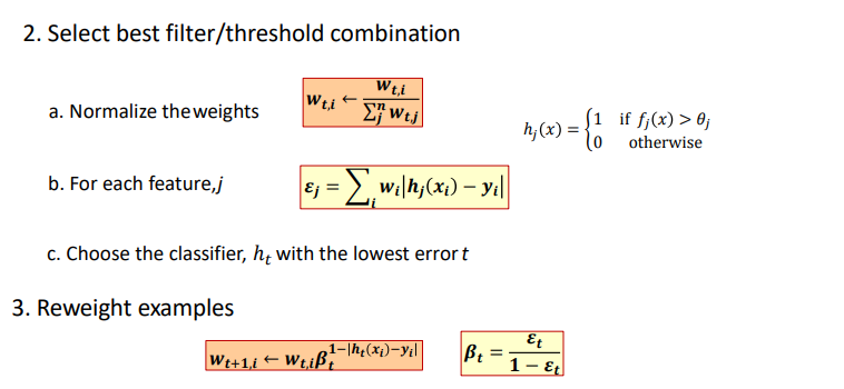
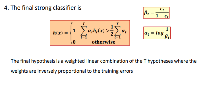
Boosting
-
Defines a classifier using an additive model 一个强分类器由多个弱分类器(线性的)组成
-
We need to define a family of weak classifiers form a family of weak classifiers
-
强弱分类器不同作用
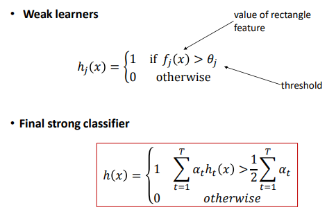
image-20220908151922789 -
人脸识别应用(Viola & Jones algorithm)
-
A “paradigmatic” method for real‐time object detection
-
Training is slow, but detection is very fast
-
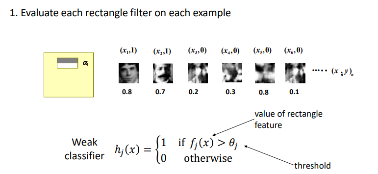
Key ideas
- Integral images 积分图 for fast feature evaluation
- Boosting for feature selection
- Attentional cascade for fast rejection of non‐face windows
-
步骤(adaboost)
-
Cascade级联分类器由多个强分类器组成
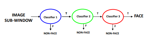
image-20220908161215860
-
-
行人检测
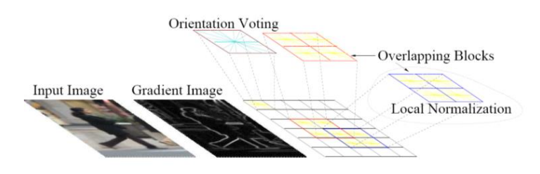
image-20220908163752127 - 步骤
- Extract fixed-sized (64x128 pixel) window at each position and scale
- Compute HOG (histogram of gradient) features within each window
- Score the window with a linear SVM classifier
- Perform non-maxima suppression to remove overlapping detections with lower scores
- 步骤
-
-
Statistical Template Approach
- Strengths
- Works very well for non-deformable objects with canonical orientations: faces, cars, pedestrians
- Fast detection
- Weaknesses
- Not so well for highly deformable objects or “stuff”
- Not robust to occlusion
- Requires lots of training data
视频(动作追踪)
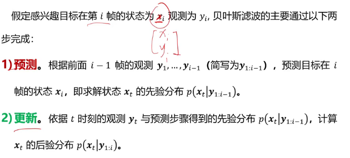
贝叶斯滤波器
-
在贝叶斯框架下,融合预测信息与有噪声的观测信息实现目标状态的估计称为贝叶斯滤波。其中,预测信息记录了目标状态的先验,观测信息表达了目标状态的似然。
-
状态通常为位置、姿态、速度、加速度等;观测通常为位置、速度等可测量,但存在噪声。
-
基本步骤
-
假设
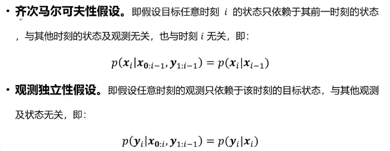
image-20220911145523156 -
递推公式
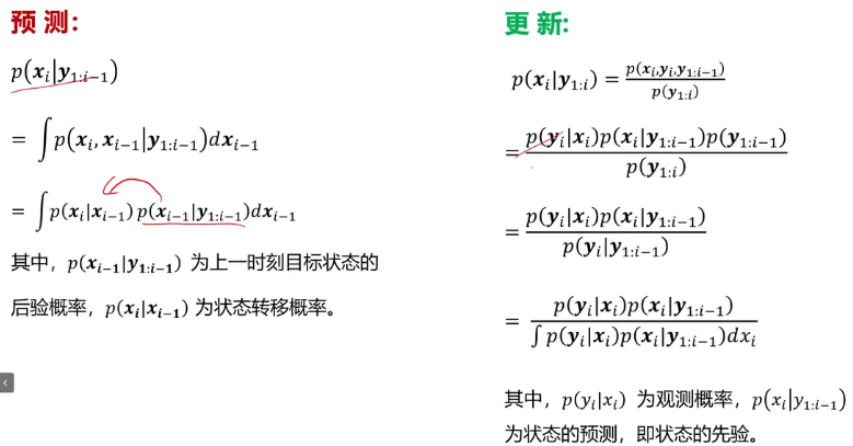
image-20220911150523440
卡曼滤波器
-
结构
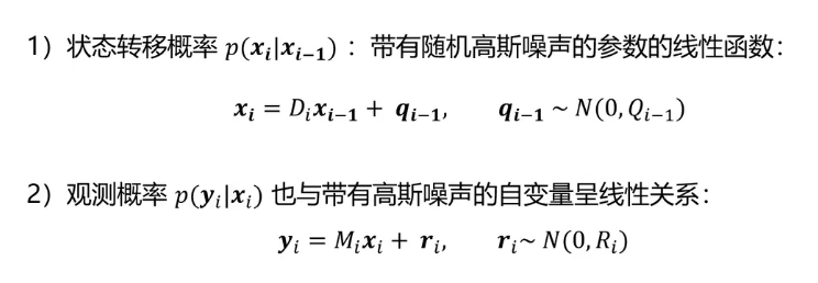
image-20220911151808123 -
略,有概率论。。。
粒子滤波器
- 太难了 以后再看 有概率论。。。
三维度量
相机
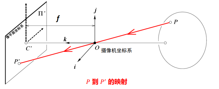
摄像机结构
-
结构
-
随着光圈减小,成像效果如何变化?(越来越清晰、越来越暗)
-
径向畸变distortion <图像像素点以畸变中心为中心点>,沿着径向产生的位置偏差,从而导致 图像中所成的像发生形变(枕形、桶形)
-
产生原因:光线在远离透镜中心的地方比靠近 中心的地方更加弯曲
-
并不是线性的变换有z 要转换
-
欧式、齐次转换
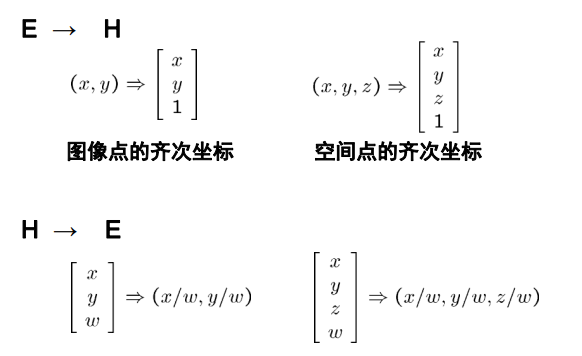
-
多个齐次可以转成一个欧式 [2,2,2] [1,1,1] -> [1,1]
-
欧式到齐次只有一个
-
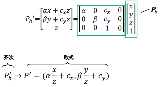
齐次坐标系中的投影变换
考虑夹角
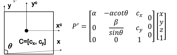
-
摄像机内参数矩阵,K有五个自由度
-
世界坐标系
-
摄像机几何关系(是相机制造内部参数, 是摄像机所处世界外部参数,有5+6=11个自由度)
-
各种摄像机模型
-
正交投影:摄像机中心到像平面的距离无限远时。更多应用在建筑设计(AUTOCAD)或者工业设计行业
-
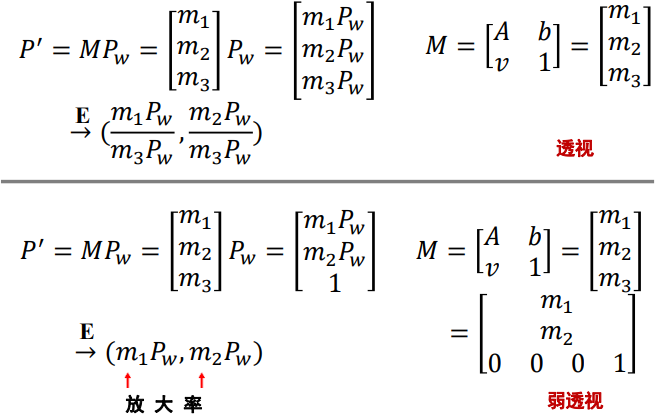
弱透视投影(当相对场景深度小于其与相机的距离时 ):在数学方面更简单 –当物体较小且较远时准确,常用于图像识别任务。
-
透视投影:对于3D到2D映射的建模更为准确 –用于运动恢复结构或SLAM
-
弱透视投影与透视投影摄像机对比
-
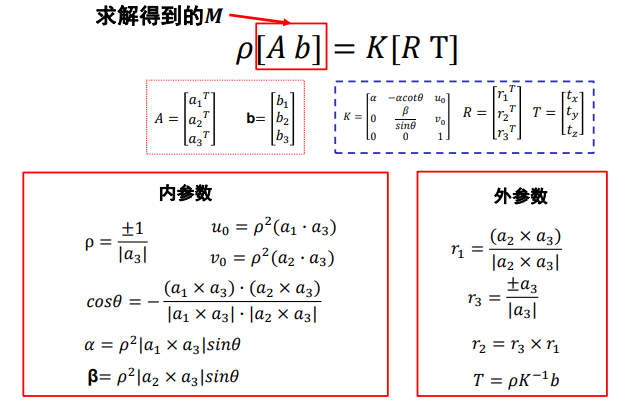
摄像机标定
-
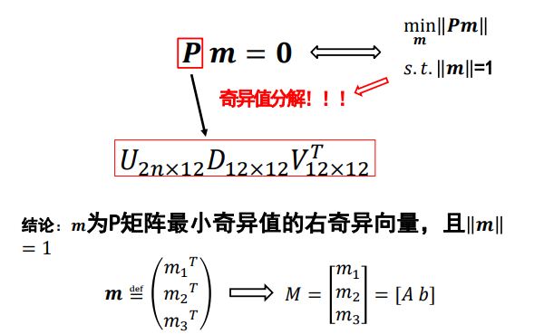
目标:从1张或多张图像中估算内外参数,11个未知量,一张照片可以两个方程,至少要六张图,来自不同平面,解方程组求m即可
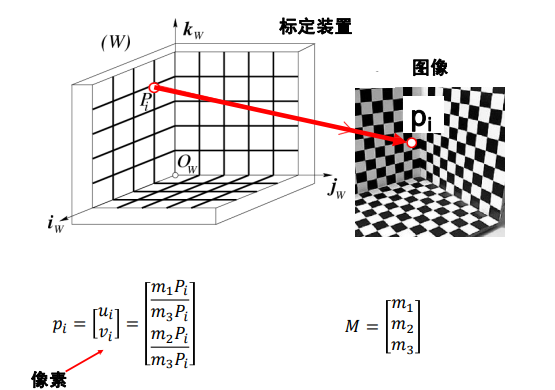
image-20220908204102483 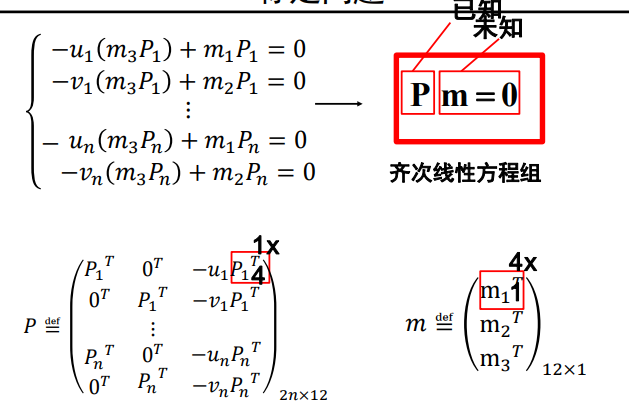
推导略
多视角几何
三个关键问题
- 摄像机几何:标定
- 场景几何:通过多幅图找到3d坐标
- 对应关系已知图像坐标p求另一图像的p’
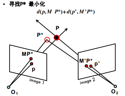
三角化
-
已知𝑝和𝑝′,𝐾和𝐾′以及𝑅,𝑇,求解:𝑃点的三维坐标?
-
使用非线性解法
极几何
-
极几何描述了同一场景或者物体的两个视点图像间的几何关系
-
对于问题“对应关系已知图像坐标p求另一图像的p’”,通过极几何约束,将搜索范围缩小到对应的极线上。
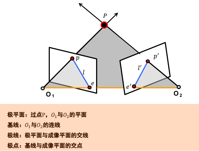
image-20220910164904185 -
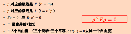
本质矩阵:本质矩阵对规范化(𝐾 = 𝐾′已知且为规范化)摄像机拍摄的两个视点图像间的极几何关系进行代数描述
-
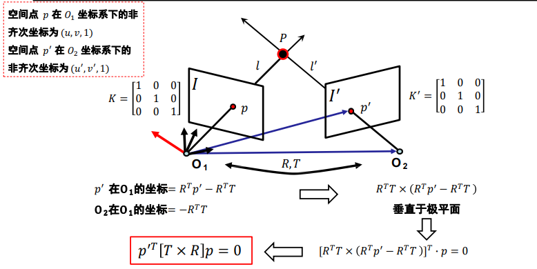
-
叉乘的矩阵表示
-
E为本质矩阵
-
基础矩阵:基础矩阵对一般的透视摄像机拍摄的两个视点的图像间的极几何关系进行代数描述,需要变换到规范化摄像机
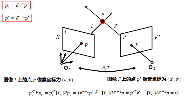
image-20220911084241239 -
F为基础矩阵
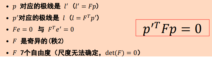
- 如果已知 ,无需场景信息以及摄像机内、外参数(他本身由参数构成),即可建立左右图像对应关系, 刻画了两幅图像的极几何关系,即相同场景在不同视图中的对应关系
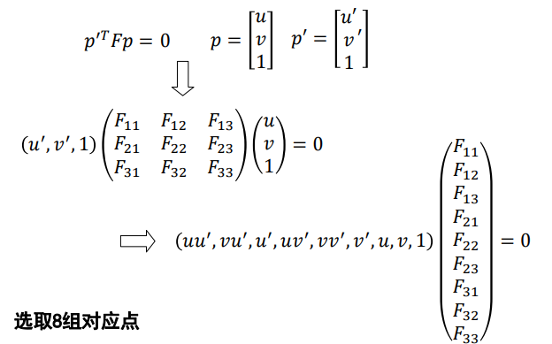
基础矩阵F估计(八点法)
-
使用八点算法,选取8组对应点,一般会选择更多点,超定
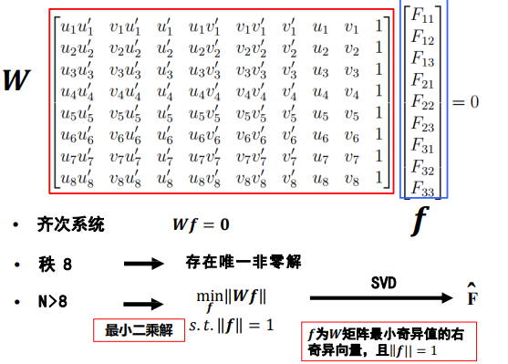
-
问题:是不是我们要求的基础矩阵? 回答:不是,基础矩阵的秩为2,通常秩为3,即满秩
-
Frobenius 范数(F-范数):矩阵中每项数的平方和的开方值
-
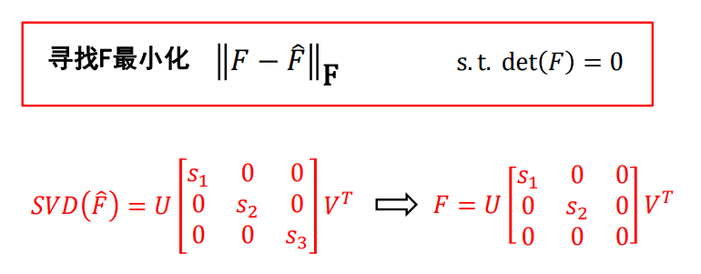
image-20220911093410432 -
问题:精度较低,W 中各个元素的数值差异过大、SVD分解有数值计算问题
-
改进:归一化八点算法
- 对每幅图像施加变换 (平移与缩放),让其满足如下条件
- 原点 = 图像上点的重心
- 各个像点到坐标原点的均方根距离等于 根号2(或者均方距离等于2)
- 步骤
- 计算左右图的变换 和
- 坐标归一化
- 计算矩阵
- 逆归一化
- 对每幅图像施加变换 (平移与缩放),让其满足如下条件
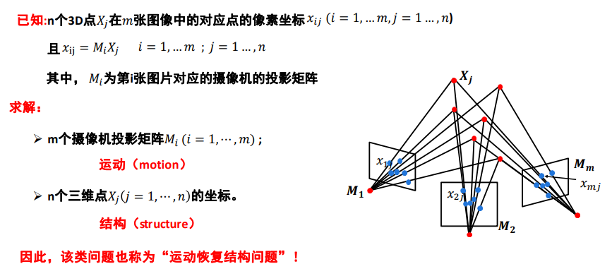
运动恢复结构
-
Structure from Motion (sfm)
-
通过三维场景的多张图像,恢复出该场景的三维结构信息以及每张图片对应的摄像机参数
-
对比:sfm没有序列,slam通常有时间序列的顺序加快算法速度
-
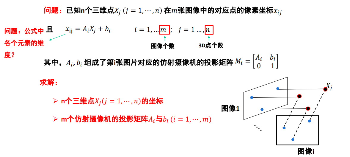
问题描述
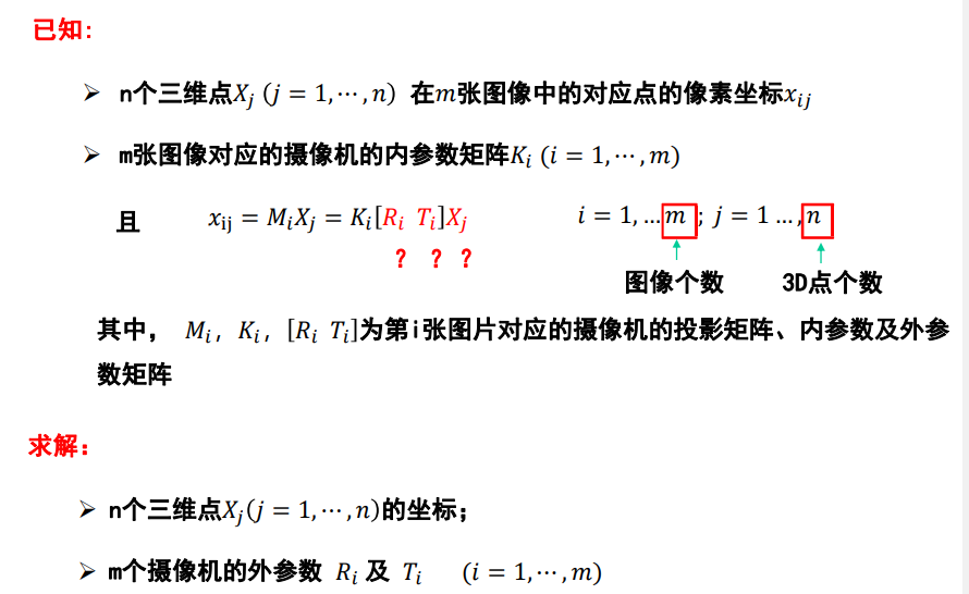
欧式结构恢复
-
摄像机内参数已知,外参数未知
-
问题描述
-
求解方法(两视图)
-
找点对(SIFT、特征匹配、RANSAC )
-
归一化八点法求解基础矩阵F
-
利用F与摄像机内参数求解本质矩阵E
-
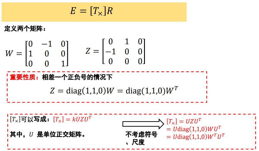
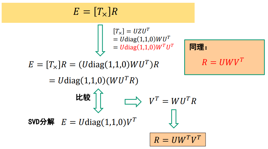
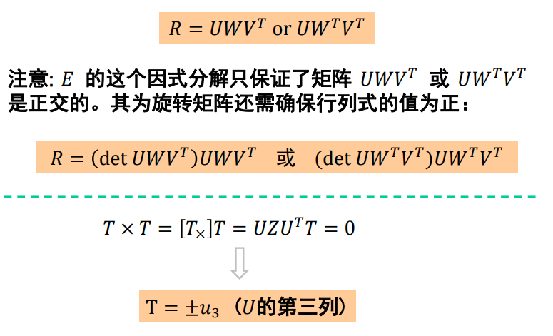
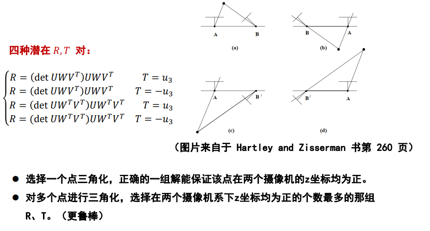
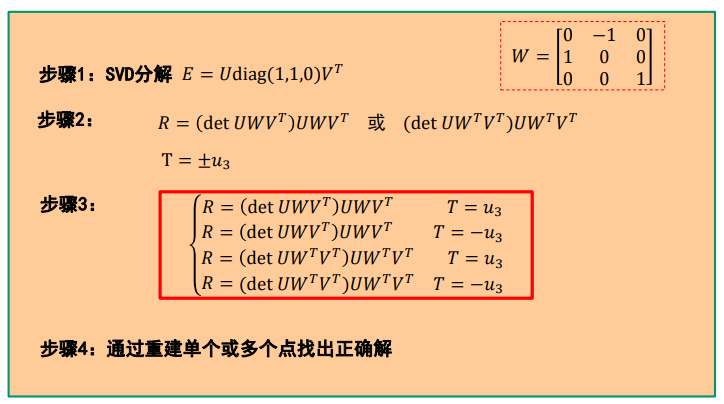
分解本质矩阵获得R与T(核心问题)
-
三角化求解三维点坐标
-
-
核心问题:分解E为R和T
- 说明:无法确定𝐹的符号及尺度,−𝐹或者𝑘𝐹都满足上式;所以,也无法确定𝐸的符号及尺度
ps: R是旋转矩阵(Rotation matrix),旋转矩阵是在乘以一个向量的时候有改变向量的方向但不改变大小的效果并保持了手性的矩阵。
-
步骤总结
-
欧式结构恢复歧义
- 需要其他先验信息,否则不能估计场景的绝对尺度
- 恢复出来的欧式结构与真实场景之间相差一个相似变换(旋转,平移,缩放),需要一个重构称为度量重构
仿射结构恢复
-
摄像机为仿射相机(忽略距离较小的深度),内、外参数均未知
-
问题描述
-
主要解法:数据中心化+因式分解
-
中心化:减去图像点的质心,当3D点的质心 = 世界坐标系的中心,此时只和A有关
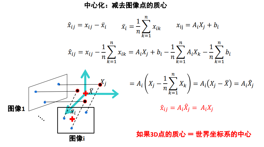
image-20220911111710940 -
因式分解
-
-
步骤总结
-
计算中心
-
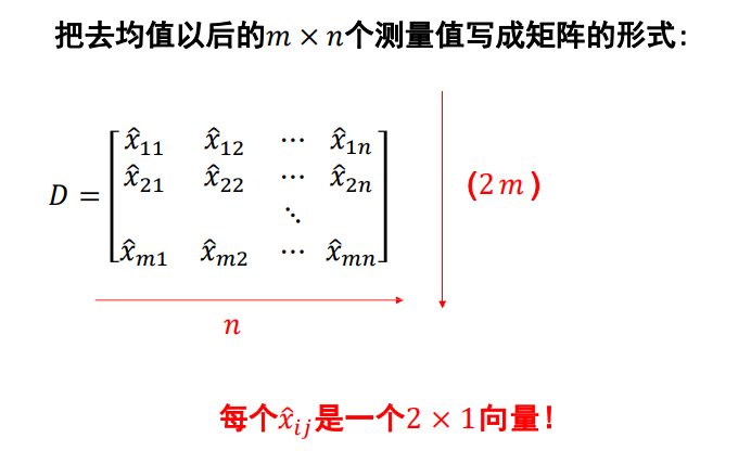
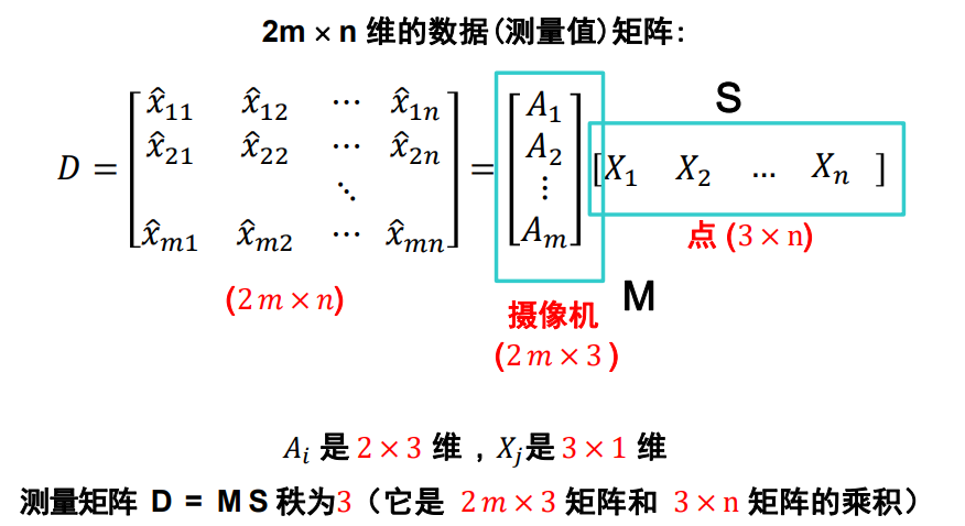
创建一个 2m x n 维的数据(测量值)矩阵D
-
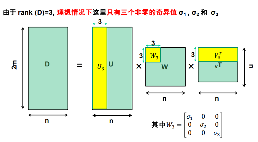
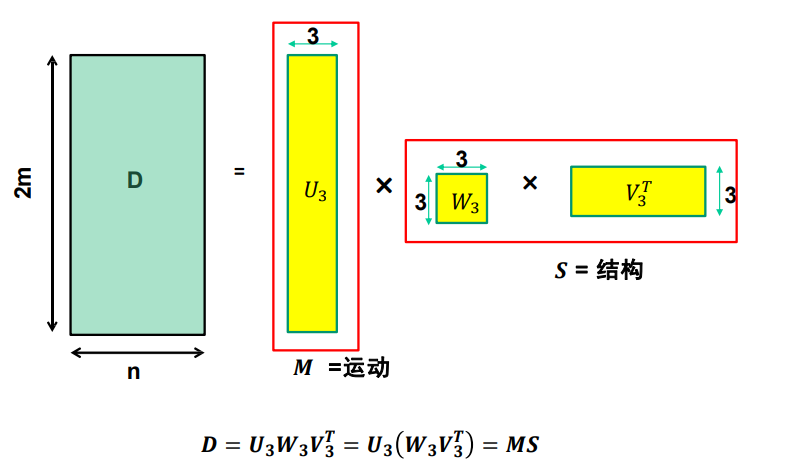
SVD分解矩阵,找最大的三个特征值,求出左上角留下的矩阵
\begin{eqnarray} D & = & U_{3} W_{3} V_{3}^{T}\\ M & = & U_{3} \\ S & = & W_{3} V_{3}^{T} \end{eqnarray}
-
-
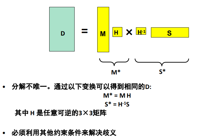
问题
-
能不能 ,行
-
引出恢复歧义:解并不是唯一的,和结果差一个3x3矩阵,8个未知量
-
可以通过角度关系直角等进行部分,将仿射升级为欧式重构
-
透视结构恢复
-
摄像机为透视相机(精算各种深度细节),内、外参数均未知
-
问题描述
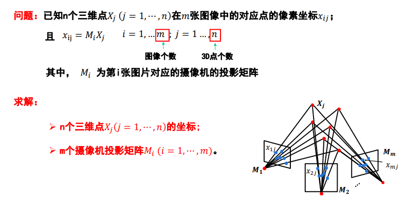
image-20220911131125494 -
透视结构恢复歧义
-
主要方法:在相差一个4×4的可逆变换的情况下恢复摄像机运动与场景结构
- 代数方法(通过基础矩阵)
- 因式分解法(通过SVD),难,复杂
- 捆绑调整
-
代数方法
-
主要步骤
-
归一化八点法求解基础矩阵 F
-
利用 F 估计摄像机矩阵M(重点)
-
三角化计算三维点坐标
-
-
利用 F 估计摄像机矩阵(两视图)
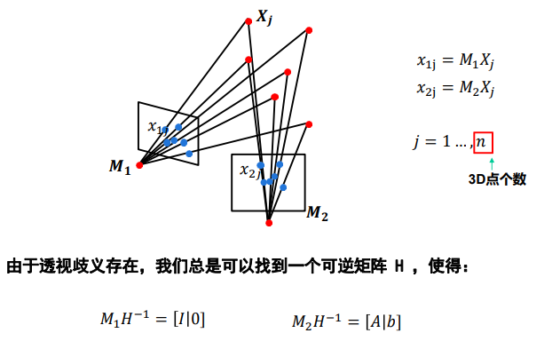
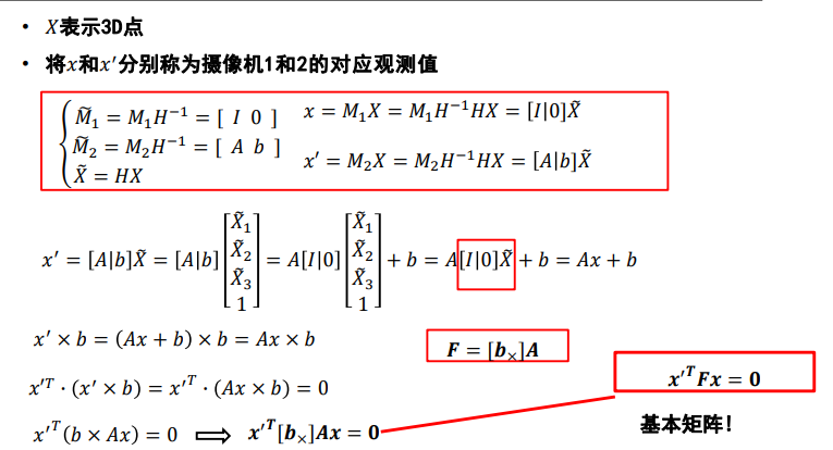
image-20220911132648474 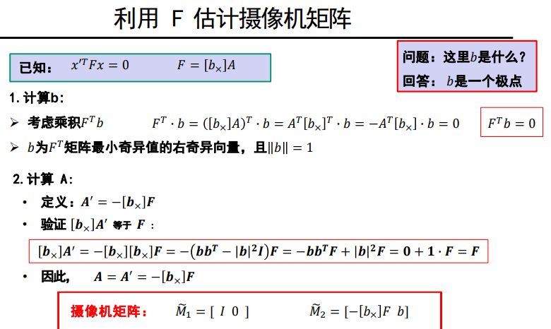
-
多视图情况:增量法,有误差,代数法缺陷
-
-
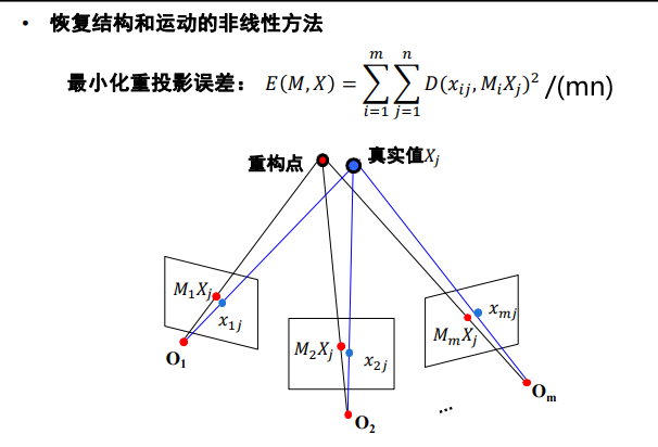
捆绑调整(Bundle Adjustment)
-
选择原因
- 因式分解法假定所有点都是可见的,所以下述场合(存在遮挡、建立对应点关系失败)的时候不可用
- 代数法应用于2视图重建,易出现误差累积
-
问题描述(非线性最小化问题)
使用的最优化方法:牛顿法 与 列文伯格-马夸尔特法(L-M方法)
-
pro
- 同时处理大量视图
- 处理丢失的数据
-
con
- 大量参数的最小化问题
- 需要良好的初始条件
-
实际操作:常用作SFM的最后一步,分解或代 数方法可作为优化问题的初始解
-
Comments