糖尿病遗传风险检测挑战赛 - Coggle 30 Days of ML（22年7月）

Jun 26, 2022

任务1：报名比赛#

步骤1：报名比赛http://challenge.xfyun.cn/topic/info?type=diabetes&ch=ds22-dw-zmt05
步骤2：下载比赛数据（点击比赛页面的赛题数据）

步骤3：解压比赛数据，并使用pandas进行读取

1
import pandas as pd
2

3
train_df = pd.read_csv('./比赛训练集.csv', encoding='gbk')
4
test_df = pd.read_csv('./比赛测试集.csv', encoding='gbk')
5

6
print(train_df.shape,test_df.shape)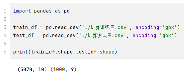

步骤4：查看训练集和测试集字段类型
```
1
train_df.dtypes
2
test_df.dtypes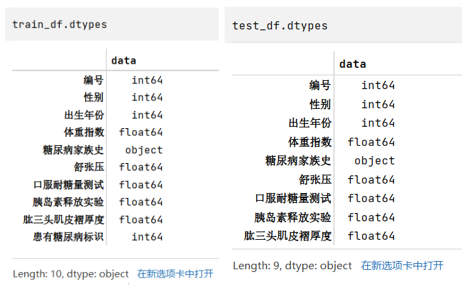
```

任务2：比赛数据分析#

步骤1：统计字段的缺失值，计算缺失比例；

通过缺失值统计，训练集和测试集的缺失值分布是否一致？
通过缺失值统计，有没有缺失比例很高的列？

1
train_nan_df = pd.DataFrame(columns=['标签','训练集缺失个数','训练集缺失比例'])
2
i = 0
3
for tag in list(train_df.columns):
4
    num = train_df[tag].isnull().sum()
5
    num_rate = num/len(train_df)
6
    train_nan_df.loc[i] = [tag, num, num_rate]
7
    i += 1
8
# train_nan_df
9

10
test_nan_df = pd.DataFrame(columns=['标签','测试集缺失个数','测试集缺失比例'])
11
i = 0
12
for tag in list(test_df.columns):
13
    num = test_df[tag].isnull().sum()
14
    num_rate = num/len(test_df)
15
    test_nan_df.loc[i] = [tag, num, num_rate]
16
    i += 1
17
# test_nan_df
18

19
train_nan_df.merge(test_nan_df,how='left')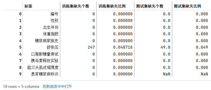

根据结果可知，训练集和测试集的缺失值分布一致，都是有且只有舒张压这一个标签含缺失值，且比例都在4.8-4.9%左右，缺失的比例其实也不算是特别高。

步骤2：分析字段的类型

有多少数值类型、类别类型？

你是判断字段类型的？

1
train_df.head() # tail()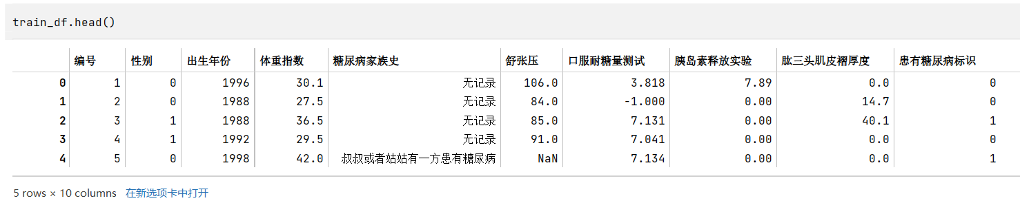

1
train_category_num_df = pd.DataFrame(columns=['标签','训练集该标签不同值个数'])
2
i = 0
3
for tag in list(train_df.columns):
4
    num = len(train_df[tag].value_counts())
5
    train_category_num_df.loc[i] = [tag, num]
6
    i += 1
7
# train_category_num_df
8

9
test_category_num_df = pd.DataFrame(columns=['标签','测试集该标签不同值个数'])
10
i = 0
11
for tag in list(test_df.columns):
12
    num = len(test_df[tag].value_counts())
13
    test_category_num_df.loc[i] = [tag, num]
14
    i += 1
15
# test_category_num_df
16

17
train_category_num_df.merge(test_category_num_df,how='left')
18
# 列包含NaN，因此dtype必须升级为浮点dtype以容纳

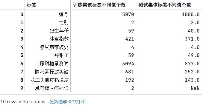
字段类型的判断主要通过根据常识（如性别）、观察原始数据（如糖尿病家族史）、以及各个标签的类型数量（如数量较多的可能就是连续性数据，是数值类型）来判断

数值类型：编号（和时序无关，后期没必要研究），出生年份，体重指数，舒张压，口服耐糖量测试，胰岛素释放实验，肱三头肌皮褶厚度
类别类型：性别（两类），糖尿病家族史（类型），患有糖尿病标识
当然，后期为了改善模型效果，也可以将一些连续性数据转换成类别，比如体重指数可以根据国家标准划分胖瘦类型，成为类别类型
其中，糖尿病家族史有四类，但是查看其类型，和“叔叔或者姑姑有一方患有糖尿病”应是同一表述，但是被分到两类，应该合并成一类为“叔叔或姑姑有一方患有糖尿病”

1
train_df.糖尿病家族史.value_counts()
2

3
train_df.loc[train_df.糖尿病家族史 == '叔叔或者姑姑有一方患有糖尿病','糖尿病家族史'] = '叔叔或姑姑有一方患有糖尿病'
4
train_df.糖尿病家族史.value_counts()
5

6
train_df['糖尿病家族史'] = train_df['糖尿病家族史'].astype('int64')
7
test_df['糖尿病家族史'] = test_df['糖尿病家族史'].astype('int64')
8
train_df.dtypes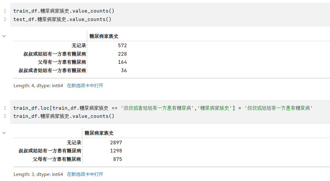

步骤3：计算字段相关性

通过.corr()计算字段之间的相关性
有哪些字段与标签的相关性最高？
尝试使用其他可视化方法将字段与标签的分布差异进行可视化

1
tag_list = train_df.columns.tolist()
2
tag_list.pop(tag_list.index("编号"))
3
corr = train_df[tag_list].corr()
4
cor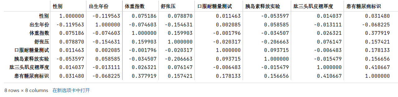r

虽然获得了相关系数矩阵，但是不便于分析结果，将其进行可视化，使用seaborn绘制热力图

1
from string import ascii_letters
2
import numpy as np
3
import pandas as pd
4
import seaborn as sns
5
import matplotlib.pyplot as plt
6

7
sns.set_theme(style="white")
8
plt.rcParams['font.sans-serif'] = ['SimHei']  # 黑体
9
plt.rcParams['axes.unicode_minus']=False # 负号
10

11
# Generate a mask for the upper triangle
12
mask = np.triu(np.ones_like(corr, dtype=bool))
13

14
# Set up the matplotlib figure
15
f, ax = plt.subplots(figsize=(8, 8))
16

17
# Generate a custom diverging colormap
18
cmap = sns.diverging_palette(230, 20, as_cmap=True)
19
# Draw the heatmap with the mask and correct aspect ratio
20
sns.heatmap(corr, mask=mask, cmap=cmap, vmax=0.5, center=0, vmin=-0.3,
21
            square=True, linewidths=2, cbar_kws={"shrink": .5})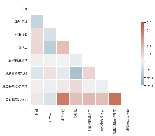

颜色越深，表示和标签的相关性最高，也就是可以重点关注一下体重指数和肱三头肌褶厚度。

同时，还对不同的自变量之间进行相关性分析，按照是否有患有糖尿病标识绘制多变量联合分布pairplot图

1
sns.set_theme(style="ticks")
2

3
plt.rcParams['font.sans-serif'] = ['SimHei']  # 黑体
4
plt.rcParams['axes.unicode_minus']=False # 负号
5

6
sns.pairplot(train_df.drop(columns=['编号','性别']), hue='患有糖尿病标识',plot_kws={'alpha': 0.5})

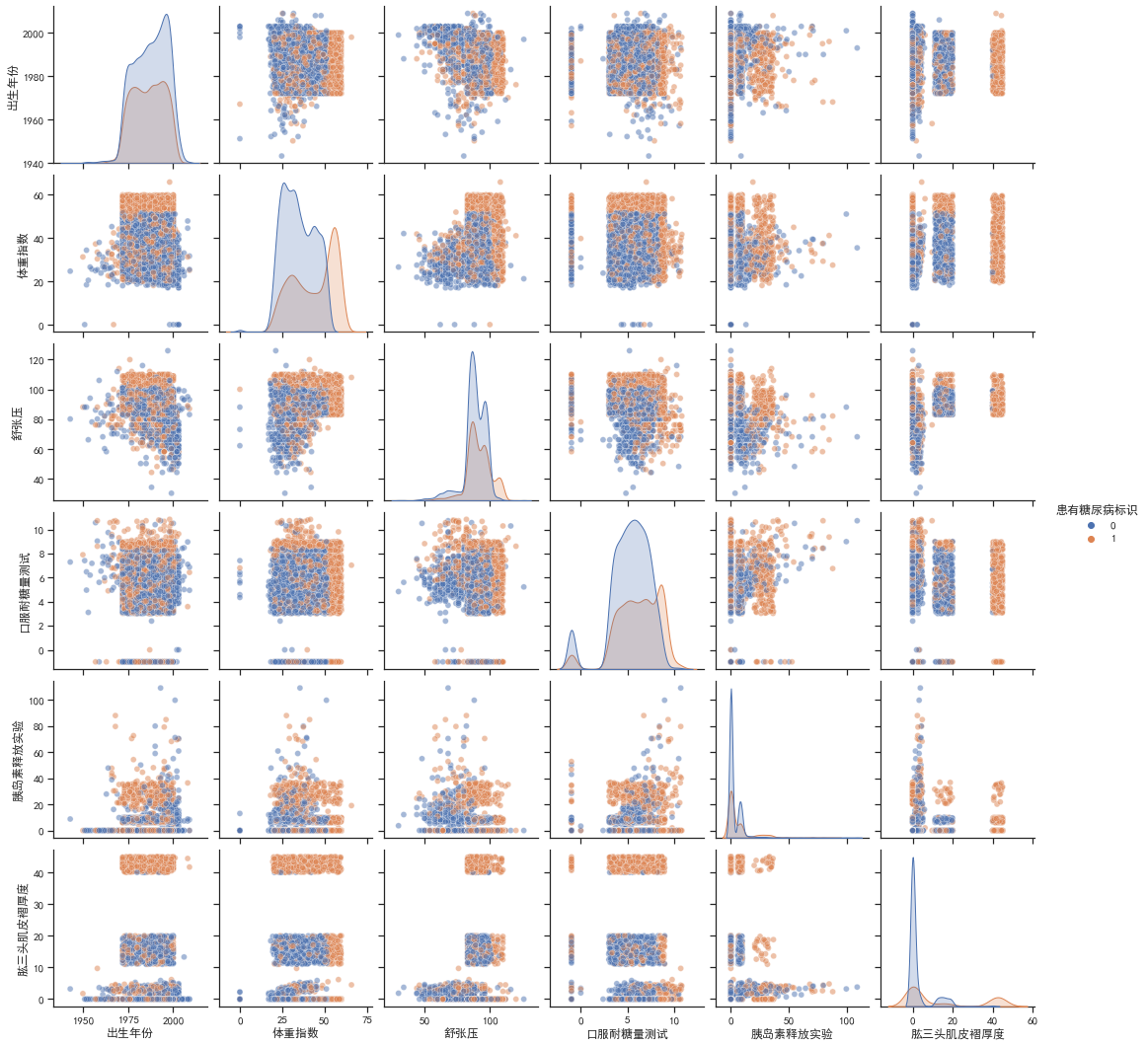
由对角线可知，患有糖尿病和非患者的体重指数和肱三头肌褶厚度的分布有较大差别，患有糖尿病的分布都略向右偏移。由其他子图可知，患者的一些联合分布特征聚集比较紧密，有一些数据还有明显的中断、不连续，可以将其作为类别特征处理，如肱三头肌褶厚度，如果在40以上就极有可能是患者，这样处理可以提高准确率。

任务3：逻辑回归尝试#

步骤1：导入sklearn中的逻辑回归；
步骤2：使用训练集和逻辑回归进行训练，并在测试集上进行预测；

1
# 预处理（文字转编码、消除nan）
2
train_df.loc[train_df.糖尿病家族史 == '无记录','糖尿病家族史'] = 0
3
train_df.loc[train_df.糖尿病家族史 == '叔叔或姑姑有一方患有糖尿病','糖尿病家族史'] = 1
4
train_df.loc[train_df.糖尿病家族史 == '父母有一方患有糖尿病','糖尿病家族史'] = 2
5

6
test_df.loc[test_df.糖尿病家族史 == '无记录','糖尿病家族史'] = 0
7
test_df.loc[test_df.糖尿病家族史 == '叔叔或者姑姑有一方患有糖尿病','糖尿病家族史'] = 1
8
test_df.loc[test_df.糖尿病家族史 == '叔叔或姑姑有一方患有糖尿病','糖尿病家族史'] = 1
9
test_df.loc[test_df.糖尿病家族史 == '父母有一方患有糖尿病','糖尿病家族史'] = 2
10

11
pressure_average = sum(train_df.loc[train_df["舒张压"].notnull(),"舒张压"].tolist())/len(train_df.loc[train_df["舒张压"].notnull()])
12
train_df.loc[train_df["舒张压"].isnull(),"舒张压"] = pressure_average
13
train_df
14

15
test_df.loc[test_df["舒张压"].isnull(),"舒张压"] = pressure_average
16
test_df
17

18
# 开始训练
19
from sklearn import linear_model
20

21
train_X, train_y = train_df.iloc[:, 1:-1].values, train_df.iloc[:, -1].values
22
test_X  = test_df.iloc[:, 1:].values
23
lr = linear_model.LogisticRegression(random_state=42, max_iter=200).fit(train_X, train_y)
24

25
# lr.predict_proba(train_X) # 可以获得每个预测的分数
26
lr.score(train_X, train_y) # 0.8122287968441815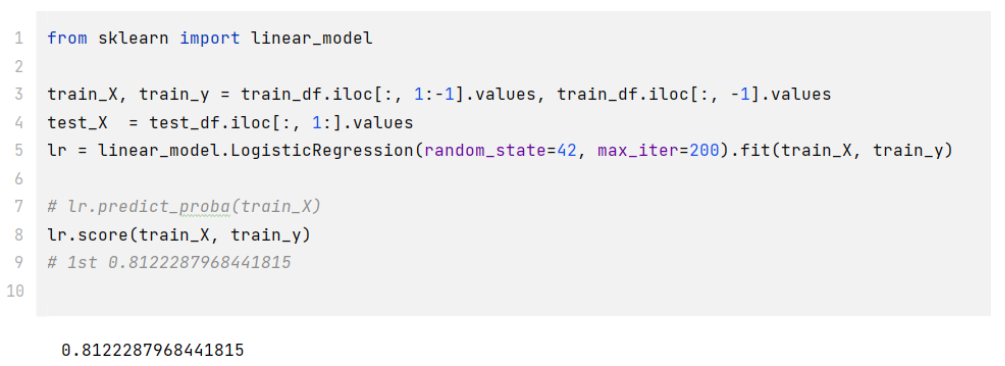

步骤3：将步骤2预测的结果文件提交到比赛，截图分数

1
df = pd.DataFrame(enumerate(test_y,1), columns=['uuid','label'])
2
df.to_csv('0713-hjy.csv', index=False)

步骤4：将训练集20%划分为验证集，在训练部分进行训练，在测试部分进行预测，调节逻辑回归的超参数

1
from sklearn.utils import shuffle
2

3
index = int(len(train_df)*0.8)
4
train_df = shuffle(train_df)
5
train_X, train_y = train_df.iloc[:index, 1:-1].values, train_df.iloc[:index, -1].values
6
val_X, val_y     = train_df.iloc[index:, 1:-1].values, train_df.iloc[index:, -1].values
7
lr1 = linear_model.LogisticRegression(random_state=42, max_iter=150, C=100).fit(train_X, train_y)
8
lr1.score(val_X, val_y)
9
# 直接分割 0.8126232741617357 0.7938856015779092 0.8353057199211046 无明显变化

步骤5：如果精度有提高，则重复步骤2和步骤3；如果没有提高，可以尝试树模型，重复步骤2、3

1
from sklearn.ensemble import RandomForestClassifier # 使用随机森林
2

3
index = int(len(train_df)*0.8)
4
train_df = shuffle(train_df)
5
train_X, train_y = train_df.iloc[:index, 1:-1].values, train_df.iloc[:index, -1].values
6
val_X, val_y     = train_df.iloc[index:, 1:-1].values, train_df.iloc[index:, -1].values
7
lr2 = RandomForestClassifier(n_estimators=50).fit(train_X, train_y) #参数50
8
lr2.score(val_X, val_y)
9
# 随机森林 0.9615384615384616 0.9575936883629191 0.9694280078895463 很可以了

提交一波

任务4：特征工程#

步骤1：统计每个性别对应的【体重指数】、【舒张压】平均值（后面重做的时候最后发现体重指数有等于0的情况，实际上没有意义，应该设置为中位数或者平均数比较合适）

1
index = int(len(train_df)*0.8)
2
train_df = shuffle(train_df)
3

4
# groupby真好用
5
woman_BMI_average, man_BMI_average = train_df.groupby('性别').mean()['体重指数']
6
woman_pressure_average, man_pressure_average = train_df.groupby('性别').mean()['舒张压']
7
woman_BMI_average, man_BMI_average, woman_pressure_average, man_pressure_average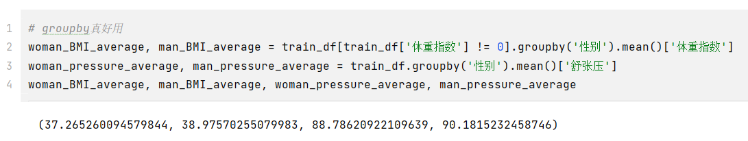

步骤2：计算每个患者与每个性别平均值的差异

1
train_df['BMI_delta'] = 0
2
train_df['pressure_delta'] = 0
3

4
for i in range(len(train_df)):
5
    if train_df.iloc[i, 1] == 0:
6
        if train_df['体重指数'][i] == 0:
7
            train_df['体重指数'][i] = woman_BMI_average
8
        train_df['BMI_delta'][i] = train_df['体重指数'][i] - woman_BMI_average
9
        train_df['pressure_delta'][i] = train_df['舒张压'][i] - woman_pressure_average
10
    else:
11
        if train_df['体重指数'][i] == 0:
12
            train_df['体重指数'][i] = man_BMI_average
13
        train_df['BMI_delta'][i] = train_df['体重指数'][i] - man_BMI_average
14
        train_df['pressure_delta'][i] = train_df['舒张压'][i] - man_pressure_average
15

16
train_df
17

18
test_df['BMI_delta'] = 0
19
test_df['pressure_delta'] = 0
20

21
for i in range(len(test_df)):
22
    if test_df.iloc[i, 1] == 0:
23
        if test_df['体重指数'][i] == 0:
24
            test_df['体重指数'][i] = woman_BMI_average
25
        test_df['BMI_delta'][i] = test_df['体重指数'][i] - woman_BMI_average
26
        test_df['pressure_delta'][i] = test_df['舒张压'][i] - woman_pressure_average
27
    else:
28
        if test_df['体重指数'][i] == 0:
29
            test_df['体重指数'][i] = man_BMI_average
30
        test_df['BMI_delta'][i] = test_df['体重指数'][i] - man_BMI_average
31
        test_df['pressure_delta'][i] = test_df['舒张压'][i] - man_pressure_average
32

33
test_df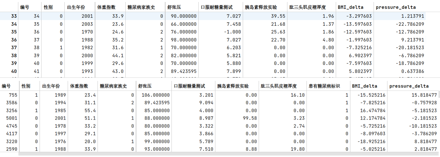

步骤3：在上述基础上将训练集20%划分为验证集，使用逻辑回归完成训练，精度是否有提高？

1
from sklearn.metrics import f1_score
2
train_y = train_df.iloc[:index, -3].values
3
val_y   = train_df.iloc[index:, -3].values
4
train_edit_df = train_df.drop(columns='患有糖尿病标识')
5
train_X = train_edit_df.iloc[:index, 1:].values
6
val_X   = train_edit_df.iloc[index:, 1:].values
7

8
test_X  = test_df.iloc[:, 1:].values
9

10
# lr3 = linear_model.LogisticRegression(random_state=42, max_iter=1000, C=100).fit(train_X, train_y)
11
# lr3.score(val_X, val_y) #0.8274161735700197 对于逻辑回归变化不大
12

13
clf2 = RandomForestClassifier(n_estimators=30).fit(train_X, train_y) #参数30
14
val_y_predict = clf2.predict(val_X)
15
# clf2.score(val_X, val_y) #0.9635108481262328
16
f1_score(val_y, val_y_predict) # 0.9488859764089121

步骤4：思考字段含义，尝试新的特征

1
from sklearn.metrics import f1_score
2

3
train_y = train_df.iloc[:index, -5].values
4
val_y = train_df.iloc[index:, -5].values
5
train_edit_df = train_df.drop(columns='患有糖尿病标识')
6
train_X = train_edit_df.iloc[:index, 1:].values
7
val_X = train_edit_df.iloc[index:, 1:].values
8

9
test_X = test_df.iloc[:, 1:].values
10

11
# lr4 = linear_model.LogisticRegression(random_state=42, max_iter=5000, C=10).fit(train_X, train_y)
12
# lr4.score(val_X, val_y) #0.8441814595660749 逻辑回归有部分提高
13

14
clf3 = RandomForestClassifier(n_estimators=50).fit(train_X, train_y)  #参数50
15
val_y_predict = clf3.predict(val_X)
16
# clf3.score(val_X, val_y)  # 0.965483234714004
17
f1_score(val_y, val_y_predict) # 0.9502617801047121
18

19
def depth_type(depth):
20
    if depth < 10:
21
        return 0
22
    elif depth < 40:
23
        return 1
24
    else:
25
        return 2
26

27
def BMI_type(bmi):
28
    if bmi <= 18.4:
29
        return 0
30
    elif bmi <= 23.9:
31
        return 1
32
    elif bmi <= 27.9:
33
        return 2
34
    else:
35
        return 3
36
# 偏瘦  <= 18.4
37
# 正常  18.5 ~ 23.9
38
# 过重  24.0 ~ 27.9
39
# 肥胖  >= 28.0
40

41
train_df['bmi_type'] = train_df['体重指数'].map(lambda x: BMI_type(x))
42
train_df['depth_type'] = train_df['肱三头肌皮褶厚度'].map(lambda x: depth_type(x))
43
train_df
44

45
test_df['bmi_type'] = test_df['体重指数'].map(lambda x: BMI_type(x))
46
test_df['depth_type'] = test_df['肱三头肌皮褶厚度'].map(lambda x: depth_type(x))
47
test_df
48

49
from sklearn.metrics import f1_score
50

51
train_y = train_df.iloc[:index, -5].values
52
val_y = train_df.iloc[index:, -5].values
53
train_edit_df = train_df.drop(columns='患有糖尿病标识')
54
train_X = train_edit_df.iloc[:index, 1:].values
55
val_X = train_edit_df.iloc[index:, 1:].values
56

57
test_X = test_df.iloc[:, 1:].values
58

59
# lr4 = linear_model.LogisticRegression(random_state=42, max_iter=5000, C=10).fit(train_X, train_y)
60
# lr4.score(val_X, val_y) #0.8353057199211046 逻辑回归有部分提高
61

62
clf3 = RandomForestClassifier(n_estimators=50).fit(train_X, train_y)  #参数50
63
val_y_predict = clf3.predict(val_X)
64
# clf3.score(val_X, val_y)  # 0.97534516765286
65
f1_score(val_y, val_y_predict) # 0.9645390070921985

任务5：特征筛选#

步骤1：使用树模型完成模型的训练，通过特征重要性筛选出Top5的特征；

1
data={'featureName':train_edit_df.columns[1:],'importances':clf2.feature_importances_.tolist()}
2
df = pd.DataFrame(data)
3
df=df.sort_values(by=['importances'],ascending=False)
4
d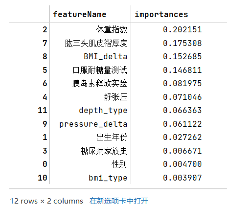f

步骤2：使用筛选出的特征和逻辑回归进行训练，在验证集精度是否有提高？

1
train_X = train_df[["体重指数","肱三头肌皮褶厚度","BMI_delta","口服耐糖量测试","胰岛素释放实验"]].iloc[:index, :].values
2
train_y = train_df["患有糖尿病标识"].iloc[:index].values
3
val_X = train_df[["体重指数","肱三头肌皮褶厚度","BMI_delta","口服耐糖量测试","胰岛素释放实验"]].iloc[index:, :].values
4
val_y =  train_df["患有糖尿病标识"].iloc[index:].values
5

6
test_X = test_df[["体重指数","肱三头肌皮褶厚度","BMI_delta","口服耐糖量测试","胰岛素释放实验"]].values
7

8
# lr5 = linear_model.LogisticRegression(random_state=42, max_iter=500, C=100).fit(train_X, train_y)
9
# lr5.score(val_X, val_y) #0.8274161735700197 逻辑回归下降了
10

11
clf4 = RandomForestClassifier(n_estimators=50).fit(train_X, train_y)  #参数50
12
val_y_predict = clf4.predict(val_X)
13
# clf4.score(val_X, val_y)  #0.9368836291913215 也下降了
14
f1_score(val_y, val_y_predict) # 0.9058823529411766

步骤3：如果有提高，为什么？如果没有提高，为什么？

没有提高，其他特征也比较重要，筛选的特征太少了导致细节丢失，换几个主要特征后，基本回升到原来的状态，应该是到了随机森林模型极限了，修改随机森林的参数也没有太大提升

1
from sklearn.metrics import f1_score
2

3
train_X = train_df[["体重指数","肱三头肌皮褶厚度","BMI_delta","口服耐糖量测试","胰岛素释放实验","舒张压","depth_type"]].iloc[:index, :].values
4
train_y = train_df["患有糖尿病标识"].iloc[:index].values
5
val_X = train_df[["体重指数","肱三头肌皮褶厚度","BMI_delta","口服耐糖量测试","胰岛素释放实验","舒张压","depth_type"]].iloc[index:, :].values
6
val_y =  train_df["患有糖尿病标识"].iloc[index:].values
7

8
test_X = test_df[["体重指数","肱三头肌皮褶厚度","BMI_delta","口服耐糖量测试","胰岛素释放实验","舒张压","depth_type"]].values
9

10
# lr6 = linear_model.LogisticRegression(random_state=42, max_iter=500, C=100).fit(train_X, train_y)
11
# lr6.score(val_X, val_y) #0.8392504930966469 没有提高
12
#
13
clf5 = RandomForestClassifier(n_estimators=50).fit(train_X, train_y)  #参数50
14
val_y_predict = clf5.predict(val_X)
15
# clf5.score(val_X, val_y)   # 0.9644970414201184
16
f1_score(val_y, val_y_predict) # 0.9501312335958005

任务6：高阶树模型#

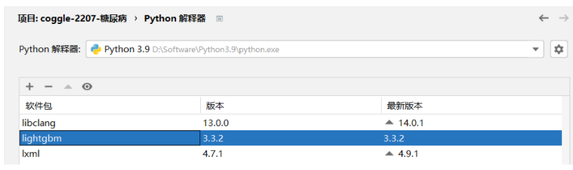
步骤1：安装LightGBM，并学习基础的使用方法

步骤2：将训练集20%划分为验证集，使用LightGBM完成训练，精度是否有提高？

1
import lightgbm as lgb
2

3
clf6 = lgb.LGBMClassifier()
4
clf6.fit(train_X, train_y, eval_set=[(val_X,val_y)], callbacks=[lgb.early_stopping(50)])
5
val_y_predict = clf6.predict(val_X)
6

7
# clf6.score(val_X, val_y)  # 0.9635108481262328
8
f1_score(val_y, val_y_predict) # 0.9512516469038208

步骤3：将步骤2预测的结果文件提交到比赛，截图分数，没有前面的好

步骤4：尝试调节搜索LightGBM的参数

1
clf7 = lgb.LGBMClassifier(
2
    max_depth=2,
3
    n_estimators=2000,
4
    n_jobs=-1,
5
    verbose=-1,
6
    learning_rate=0.2,
7
)
8
clf7.fit(train_X, train_y, eval_set=[(val_X,val_y)], callbacks=[lgb.early_stopping(50)])
9
val_y_predict = clf7.predict(val_X)
10

11
# clf7.score(val_X, val_y)  # 0.960552268244576
12
f1_score(val_y, val_y_predict) # 0.9468085106382979

步骤5：将步骤4调参之后的模型从新训练，将最新预测的结果文件提交到比赛，寄

任务7：多折训练与集成#

步骤1：使用KFold完成数据划分

1
from sklearn.model_selection import KFold
2

3
train_X = train_df[["体重指数","肱三头肌皮褶厚度","BMI_delta","口服耐糖量测试","胰岛素释放实验","舒张压","depth_type"]].iloc[:index, :]
4
train_y = train_df["患有糖尿病标识"].iloc[:index]
5
val_X = train_df[["体重指数","肱三头肌皮褶厚度","BMI_delta","口服耐糖量测试","胰岛素释放实验","舒张压","depth_type"]].iloc[index:, :]
6
val_y =  train_df["患有糖尿病标识"].iloc[index:]
7

8
test_X = test_df[["体重指数","肱三头肌皮褶厚度","BMI_delta","口服耐糖量测试","胰岛素释放实验","舒张压","depth_type"]]
9

10

11
# 模型交叉验证
12
def run_model_cv(model, kf, X_tr, y, X_te, cate_col=None):
13
    train_pred = np.zeros( (len(X_tr), len(np.unique(y))) )
14
    test_pred = np.zeros( (len(X_te), len(np.unique(y))) )
15

16
    cv_clf = []
17
    for tr_idx, val_idx in kf.split(X_tr, y):
18
        x_tr = X_tr.iloc[tr_idx]; y_tr = y.iloc[tr_idx]
19
        x_val = X_tr.iloc[val_idx]; y_val = y.iloc[val_idx]
20
        call_back = [lgb.early_stopping(50),]
21
        eval_set = [(x_val, y_val)]
22
        model.fit(x_tr, y_tr, eval_set=eval_set, callbacks=call_back)
23
        cv_clf.append(model)
24
        train_pred[val_idx] = model.predict_proba(x_val)
25
        test_pred += model.predict_proba(X_te)
26

27
    test_pred /= kf.n_splits
28
    return train_pred, test_pred, cv_clf
29

30
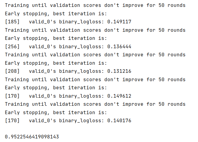
train_pred, test_pred, cv_clf = run_model_cv(
31
    clf7, KFold(n_splits=7),
32
    train_X,
33
    train_y,
34
    val_X,
35
)
36
# test_pred
37

38
test_pred_arg_max = [ i.argmax() for i in test_pred]
39
f1_score(val_y, val_y_predict) # 0.9522546419098143 没变

步骤2：使用StratifiedKFold完成数据划分

1
from sklearn.model_selection import StratifiedKFold
2

3
train_pred, test_pred, cv_clf = run_model_cv(
4
    clf8, StratifiedKFold(n_splits=10),
5
    train_X,
6
    train_y,
7
    val_X,
8
)
9
# test_pred
10

11
test_pred_arg_max = [ i.argmax() for i in test_pred]
12
f1_score(val_y, val_y_predict) # 0.9522546419098143

步骤3：使用StratifiedKFold配合LightGBM完成模型的训练和预测（如上）
步骤4：在步骤3训练得到了多少个模型，对测试集多次预测，将最新预测的结果文件提交到比赛，截图分数，分数没有增长就不截图了

步骤5：使用交叉验证训练5个机器学习模型（svm、lr等），使用stacking完成集成，将最新预测的结果文件提交到比赛，截图分数

1
from sklearn.ensemble import ExtraTreesClassifier, AdaBoostClassifier, GradientBoostingClassifier
2

3

4
#使用random forest、extratrees、adaboost、gradientboosting、svm作为第一层分类器
5
#第二层lgb
6

7
# Class to extend the Sklearn classifier
8
class SklearnHelper(object):
9
    def __init__(self, clf, seed=42, params=None):
10
        params['random_state'] = seed
11
        self.clf = clf(**params)
12

13
    def train(self, x_train, y_train):
14
        self.clf.fit(x_train, y_train)
15

16
    def predict(self, x):
17
        return self.clf.predict(x)
18

19
    def fit(self,x,y):
20
        return self.clf.fit(x,y)
21

22
    def feature_importances(self,x,y):
23
        print(self.clf.fit(x,y).feature_importances_)
24

25

26
#底层模型交叉训练oof
27

28
def get_oof(model, kf, X_tr, y, X_te, cate_col=None):
29
    train_pred = np.zeros( (len(X_tr), ))
30
    test_pred = np.zeros( (len(X_te), ))
31
    cv_clf = []
32
    for tr_idx, val_idx in kf.split(X_tr, y):
33
        x_tr = X_tr.iloc[tr_idx]; y_tr = y.iloc[tr_idx]
34

35
        x_val = X_tr.iloc[val_idx]; y_val = y.iloc[val_idx]
36

37
        model.fit(x_tr, y_tr)
38

39
        cv_clf.append(model)
40

41
        train_pred[val_idx] = model.predict(x_val)
42
        test_pred += model.predict(X_te)
43

44

45
    test_pred /= kf.n_splits
46
    return train_pred, test_pred
47

48

49
# Put in our parameters for said classifiers
50
# Random Forest parameters
51
rf_params = {
52
    'n_estimators': 100,
53
    'max_depth': 10,
54
    'min_samples_leaf': 10,
55
    'max_features' : 'sqrt',
56
}
57

58
# Extra Trees Parameters
59
et_params = {
60
    'n_jobs': -1,
61
    'n_estimators':500,
62
    'max_depth': 10,
63
    'min_samples_leaf': 10,
64
}
65

66
# AdaBoost parameters
67
ada_params = {
68
    'n_estimators': 500,
69
    'learning_rate' : 0.015
70
}
71

72
# Gradient Boosting parameters
73
gb_params = {
74
    'n_estimators': 500,
75
    'max_depth': 3,
76
    'min_samples_leaf': 2,
77
    'learning_rate': 0.015
78
}
79

80
# Support Vector Classifier parameters
81
# svc_params = {
82
#     'kernel' : 'linear',
83
#     'C' : 0.02
84
#     }
85

86

87
# Create 5 objects that represent our 5 models
88
rf =  SklearnHelper(clf=RandomForestClassifier, seed=2022,     params=rf_params)
89
et =  SklearnHelper(clf=ExtraTreesClassifier, seed=2022,       params=et_params)
90
ada = SklearnHelper(clf=AdaBoostClassifier, seed=2022,         params=ada_params)
91
gb =  SklearnHelper(clf=GradientBoostingClassifier, seed=2022, params=gb_params)
92
# svc = SklearnHelper(clf=SVC, seed=2022,                        params=svc_params)
93

94

95
# Create our OOF train and test predictions. These base results will be used as new features
96
kf = KFold(n_splits=5)
97

98
rf_oof_train, rf_oof_test =   get_oof(rf, kf, train_X, train_y, val_X) # Random Forest
99
et_oof_train, et_oof_test =   get_oof(et, kf, train_X, train_y, val_X) # Extra Trees
100
ada_oof_train, ada_oof_test = get_oof(ada,kf, train_X, train_y, val_X) # AdaBoost
101
gb_oof_train, gb_oof_test =   get_oof(gb, kf, train_X, train_y, val_X) # Gradient Boost
102
# svc_oof_train, svc_oof_test = get_oof(svc,kf, train_X, train_y, val_X) # Support Vector Classifier
103

104
print("Training is complete")
105

106
#第二层的训练及验证数据
107
base_predictions_train = pd.DataFrame({
108
    'RandomForest':  rf_oof_train.ravel(),
109
    'ExtraTrees':    et_oof_train.ravel(),
110
    'AdaBoost':      ada_oof_train.ravel(),
111
    'GradientBoost': gb_oof_train.ravel(),
112
    # 'Svc':           svc_oof_train.ravel()
113
})
114

115
base_predictions_test = pd.DataFrame({
116
    'RandomForest':  rf_oof_test.ravel(),
117
    'ExtraTrees':    et_oof_test.ravel(),
118
    'AdaBoost':      ada_oof_test.ravel(),
119
    'GradientBoost': gb_oof_test.ravel(),
120
    # 'Svc':           svc_oof_test.ravel()
121
})
122

123

124
clf8 = lgb.LGBMClassifier(
125
    # boosting_type='gbdt',
126
    # objective='binary',
127
    # metrics='binary_logloss',
128
    # learning_rate=0.015,
129
    # n_estimators=500,
130
    # max_depth=3,
131
    # num_leaves=10,
132
    # max_bin=200,
133
    # min_data_in_leaf=101,
134
    # bagging_fraction=0.8,
135
    # bagging_freq= 0,
136
    # feature_fraction= 0.8,
137
    # lambda_l1=0.7,
138
    # lambda_l2=0.7,
139
    # min_split_gain=0.1,
140
)
141

142
clf8.fit(base_predictions_train, train_y)
143
f1_score(clf8.predict(base_predictions_test),val_y)
144
# test_df['label'] = clf.predict(base_predictions_test)
145
# test_df.rename({'编号': 'uuid'}, axis=1)[['uuid', 'label']].to_csv('submit.csv', index=None)
146

147
#

改

1
from sklearn.ensemble import ExtraTreesClassifier, AdaBoostClassifier, GradientBoostingClassifier
2

3

4
#使用random forest、extratrees、adaboost、gradientboosting、svm作为第一层分类器
5
#第二层lgb
6

7

8
train_X = train_df[["体重指数","肱三头肌皮褶厚度","BMI_delta","口服耐糖量测试","胰岛素释放实验","舒张压","depth_type"]]
9
train_y = train_df["患有糖尿病标识"]
10

11
test_X = test_df[["体重指数","肱三头肌皮褶厚度","BMI_delta","口服耐糖量测试","胰岛素释放实验","舒张压","depth_type"]].iloc[:]
12

13

14
kf = KFold(n_splits=5)
15

16
rf_oof_train, rf_oof_test =   get_oof(rf, kf, train_X, train_y, test_X) # Random Forest
17
et_oof_train, et_oof_test =   get_oof(et, kf, train_X, train_y, test_X) # Extra Trees
18
ada_oof_train, ada_oof_test = get_oof(ada,kf, train_X, train_y, test_X) # AdaBoost
19
gb_oof_train, gb_oof_test =   get_oof(gb, kf, train_X, train_y, test_X) # Gradient Boost
20
# svc_oof_train, svc_oof_test = get_oof(svc,kf, train_X, train_y, val_X) # Support Vector Classifier
21

22
print("Training is complete")
23

24
#第二层的训练及验证数据
25
base_predictions_train = pd.DataFrame({
26
    'RandomForest':  rf_oof_train.ravel(),
27
    'ExtraTrees':    et_oof_train.ravel(),
28
    'AdaBoost':      ada_oof_train.ravel(),
29
    'GradientBoost': gb_oof_train.ravel(),
30
    # 'Svc':           svc_oof_train.ravel()
31
})
32

33
base_predictions_test = pd.DataFrame({
34
    'RandomForest':  rf_oof_test.ravel(),
35
    'ExtraTrees':    et_oof_test.ravel(),
36
    'AdaBoost':      ada_oof_test.ravel(),
37
    'GradientBoost': gb_oof_test.ravel(),
38
    # 'Svc':           svc_oof_test.ravel()
39
})
40

41

42
clf9 = lgb.LGBMClassifier()
43

44
clf9.fit(base_predictions_train, train_y)
45
test_y = clf9.predict(base_predictions_test)
46
test_y
47

48
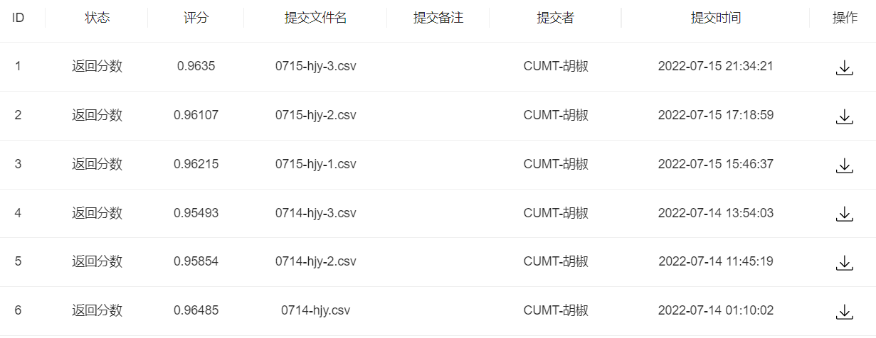
df = pd.DataFrame(enumerate(test_y,1), columns=['uuid','label'])
49
df.to_csv('0715-hjy-3.csv', index=False)

蚌埠住了，集成学习了之后还没不集成和不特征工程的分数高，傻了。

Author Junyao Hu

Published Jun 26, 2022

Link https://junyaohu.github.io/blog/30days-of-ml-202207/