《动手学深度学习》笔记

参考资料

书籍：https://zh-v2.d2l.ai/

视频：https://www.bilibili.com/video/BV1eZ4y1w7PY

ppt：https://courses.d2l.ai/zh-v2/

前言

预备知识

数据操作

预处理

线代

各种乘积

# dot product
torch.dot(x, y)

# matrix-vector product
torch.mv(A, x) 

# matrix-vector product
torch.mm(A, B)

# Hadamard product
A * B

• 各种求导

微积分

基础知识，略

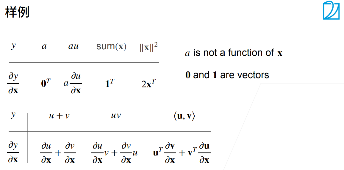
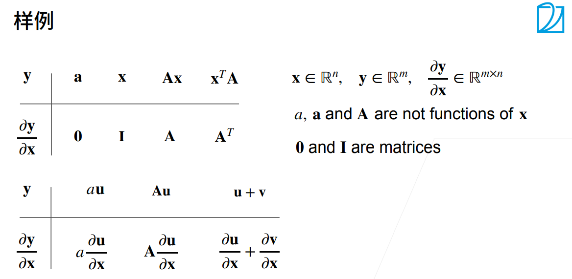
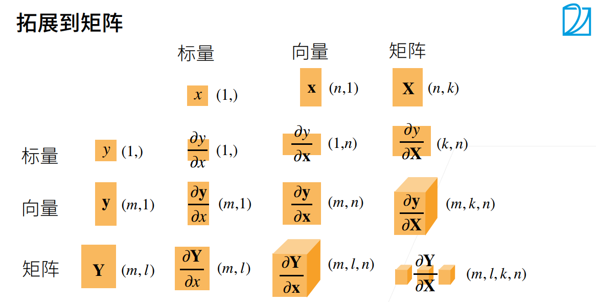
自动微分

• 在指定值上的导数，不同于符号求导和数值求导

• automatic differentiation

• 涉及到 computational graph 和 backpropagate

• 为什么DL耗资源原因之一：反向传播求梯度需要存储正向所有中间结果，复杂度 O(n)

• 非标量变量的反向传播一般是单独计算批量中每个样本的偏导数之和

import torch

x = torch.arange(4.0)
x.requires_grad_(True)  # 等价于x=torch.arange(4.0,requires_grad=True)
x.grad  # 默认值是None
y = 2 * torch.dot(x, x)
y.backward()
x.grad
# tensor([ 0., 4., 8., 12.])

x.grad.zero_()
y = x * x
# 等价于y.backward(torch.ones(len(x)))
y.sum().backward()
x.grad
# tensor([0., 2., 4., 6.])

概率

• Bayes’ theorem
• joint distribution
• conditional distribution
• marginal distribution

线性神经网络

线性回归

• linear regression

• analytical solution $\mathbf{w}^* = (\mathbf X^\top \mathbf X)^{-1}\mathbf X^\top \mathbf{y}$

• 线性回归是对n维输入的加权，外加偏差

• 使用平方损失来衡量预测值和真实值的差异
• 线性回归有显式解
• 线性回归可以看做是单层神经网络
• 梯度下降通过不断沿着反梯度方向更新参数求解
• 小批量随机梯度下降是深度学习默认的求解算法
• 两个重要的超参数是批量大小和学习率

softmax

• $\hat{\mathbf{y}} = \mathrm{softmax}(\mathbf{o})\quad \text{其中}\quad \hat{y}_j = \frac{\exp(o_j)}{\sum_k \exp(o_k)}$

• $\partial{o_j} l(\mathbf{y}, \hat{\mathbf{y}}) = \frac{\exp(o_j)}{\sum{k=1}^q \exp(o_k)} - y_j = \mathrm{softmax}(\mathbf{o})_j - y_j$

• 尽管softmax是一个非线性函数，但softmax回归的输出仍然由输入特征的仿射变换决定。 因此，softmax回归是一个线性模型（linear model）。

• 熵（entropy）

• $H[P] = \sum_j - P(j) \log P(j).$

• 可以从两方面来考虑交叉熵（cross-entropy loss）分类目标： （i）最大化观测数据的似然；（ii）最小化传达标签所需的惊异。

• 损失函数：L1，L2，Huber

• LogSumExp类似技巧

  $\begin{split}\begin{aligned}
  \log{(\hat y_j)} & = \log\left( \frac{\exp(o_j - \max(o_k))}{\sum_k \exp(o_k - \max(o_k))}\right) \
  & = \log{(\exp(o_j - \max(o_k)))}-\log{\left( \sum_k \exp(o_k - \max(o_k)) \right)} \
  & = o_j - \max(o_k) -\log{\left( \sum_k \exp(o_k - \max(o_k)) \right)}.
  \end{aligned}\end{split}$

• 单层线性无法识别XOR
• multilayer perceptrons 使用 hidden layer 和 activation function 来得到非线性模型
• sigmoid、tanh、ReLu（rectified linear unit）
• softmax处理多分类

• underfitting & overfitting
• 对抗过拟合的技术称为正则化（regularization）

• weight decay
• L1：lasso regression: 偏向于在大量特征上均匀分布权重的模型
• L2：ridge regression: 会导致模型将权重集中在一小部分特征上， 而将其他权重清除为零